Koordinates API for R

1 The problem

Many government agencies¹ in New Zealand provide spatial and tabular data through data services built on the fantastic Koordinates platform. The challenge arises when trying to import this data into R, as it involves several steps:

1. Add the dataset to your cart
2. Create an export
3. Wait for file to finish processing
4. Download the file to your computer
5. Open R
6. Navigate to the file path of the downloaded folder (e.g., in read_csv() or read_sf())
7. Finally, read the file into R.

By utilising an API, we can bypass many of these steps and read a dataset directly into R. Additionally, using an API provides the benefit of accessing the most up-to-date data, facilitating collaboration, and using version control without the need to share data files.

2 Koordinatr

I have developed a package that simplifies this process. It only works for tabular and vector spatial data for now (a function for rasters has not been implemented yet). However, it has been a time-saver for me in my work with these data.

Warning

Note: This package is still experimental, and changes may occur in the future. The arguments might change, or the whole thing might break. Use at your own risk.

2.1 Setup

2.1.1 Installation

The package is not yet available on CRAN, so it can be installed from GitHub:

# install.packages("devtools")
devtools::install_github("isaacbain/koordinatr")

2.1.2 Authentication

You will need an API key to access the data. This can be obtained by signing up on the Koordinates platform and creating a new API key.

api_key <- "your_api_key"

2.2 Usage

The package has two primary functions: get_table_as_tibble() and get_table_as_sf(). The former is for tabular data, while the latter is for spatial data.

Both functions share the same arguments:

• api_key - Your Koordinates API key.
• agency - The agency providing the data. Should be one of “linz”, “statsnz”, “mfe”. Or “custom” if you want to manually specify the URL for the service.
• id - The ID of the dataset you want to access.
• custom_url - If you set agency = "custom", you can specify the URL of the service here.

3 Example

Let’s demonstrate its use by fetching a table of greenhouse gas concentrations from the Baring Head Atmospheric Research Station, from the Ministry for the Environment data service. Using the Koordinatr package, we can directly read this data into R without manual downloading.

# libraries
library(koordinatr)
library(tidyverse)
library(gganimate)

# import data
all_gases_raw <- get_table_as_tibble(
  api_key = api_key, # set your own api key
  agency = "mfe", # set the agency
  id = "115974" # get the ID from the URL of the dataset
)

It was as easy as that! (hopefully).

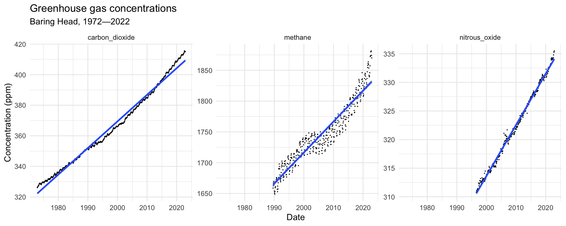
Now, let’s create a basic plot (Figure 1) using this data to check it has worked properly.

# filtering
co2 <- all_gases_raw |>
  select(-gml_id) |> # don't need this column
  filter(parameter == "trend", variable == "carbon_dioxide") |> # can select raw data points, seasonally adjusted, or the trend
  mutate(date = make_date(year = year, month = month, day = 1)) # turn columns into a proper date

all_gases <- all_gases_raw |>
  select(-gml_id) |>
  filter(parameter == "mean_fitted") |>
  mutate(date = make_date(year = year, month = month, day = 1))

ggplot(data = all_gases, aes(x = date, y = value)) +
  geom_point(size = 0.01) +
  geom_smooth(method = "lm") +
  facet_wrap(~variable, scales = "free_y") +
  theme_minimal() +
  labs(
    x = "Date",
    y = "Concentration (ppm)",
    title = "Greenhouse gas concentrations",
    subtitle = "Baring Head, 1972—2022"
  )

Figure 1: Concentration of carbon dioxide, methane, and nitrous oxide gases at Baring Head. Starting at 1972, 1990, and 1996, respectively.

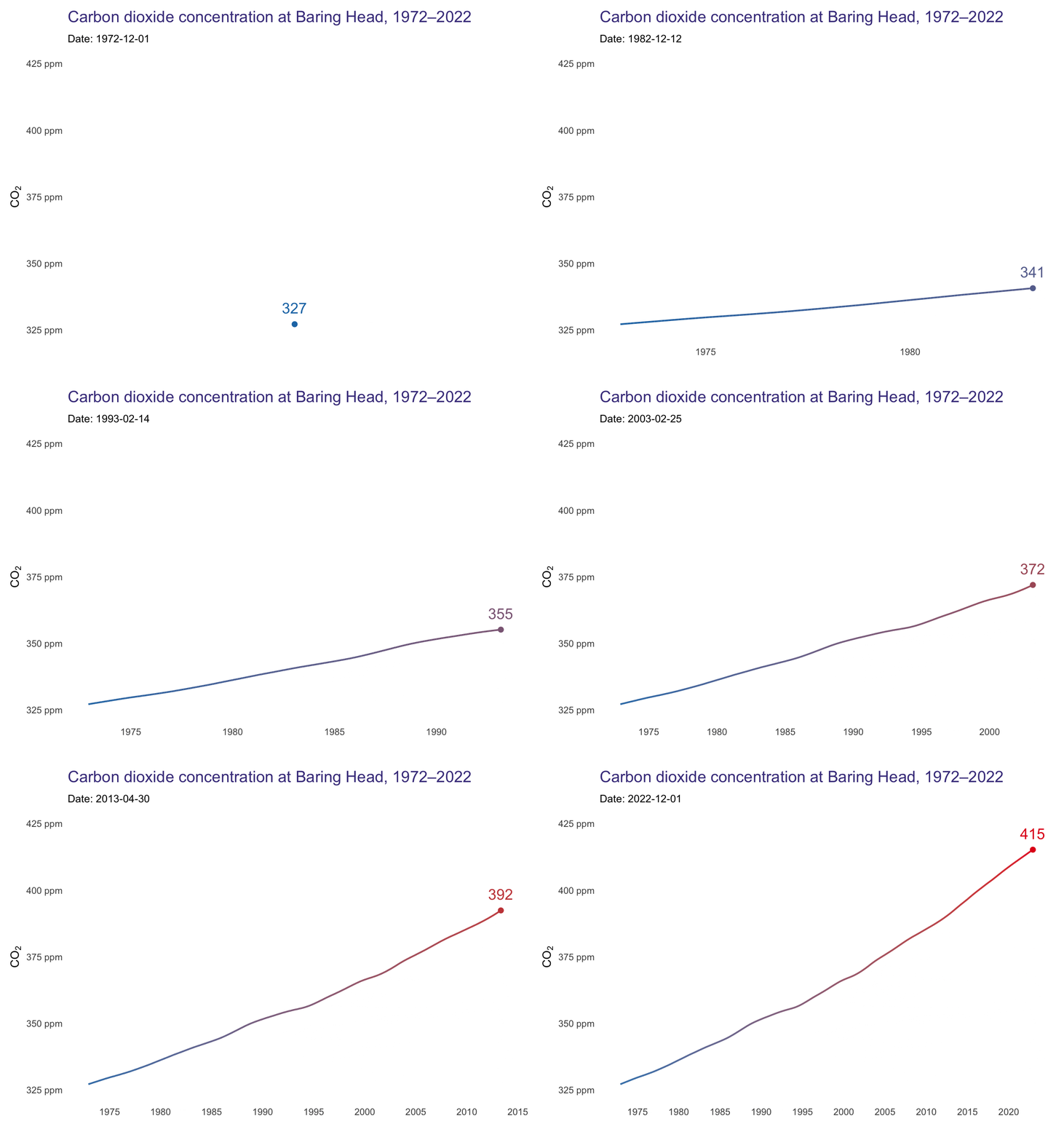
And how about an animated plot?

# Define the exact breaks for the x-axis
breaks <- seq.Date(from = as.Date("1970-01-01"), to = as.Date("2022-01-01"), by = "5 years")

# Custom labelling function
ppm_label <- function(x) {
  paste0(x, " ppm")
}

p <- ggplot(co2, aes(x = date, y = value, colour = value)) +
  geom_line(linewidth = 0.75) +
  geom_point(aes(colour = value), size = 2) +
  scale_colour_gradient(low = "#1f78b4", high = "#e31a1c") +
  transition_reveal(date) +
  expand_limits(y = c(325, 425)) +
  theme_minimal() +
  scale_y_continuous(labels = ppm_label) +
  labs(
    x = "",
    y = bquote(CO[2]),
    title = "Carbon dioxide concentration at Baring Head, 1972–2022",
    subtitle = "Date: {frame_along}"
  ) +
  theme(
    legend.position = "none",
    plot.margin = margin(t = 10, r = 10, b = 30, l = 10),
    panel.grid.major = element_blank(), # Remove major gridlines
    panel.grid.minor = element_blank(), # Remove minor gridlines
    plot.title = element_text(size = 15, face = "bold", colour = "darkslateblue"),
    plot.subtitle = element_text(size = 10)
  ) +
  geom_text(aes(label = round(value, 0), y = value), hjust = 0.5, vjust = -1, size = 5) +
  view_follow(fixed_y = TRUE) +
  scale_x_date(breaks = breaks, date_labels = "%Y", limits = range(co2$date))

animate(p,
  nframes = 400,
  fps = 30,
  start_pause = 0,
  end_pause = 60
)

Figure 2: Animated plot of carbon dioxide concentrations at Baring Head, 1972—2022.

4 Conclusion

And that’s it! You’ve now got a basic understanding of how to use the Koordinatr package to access data from the Koordinates API. These data services are a treasure trove of environmental information, so I encourage you to explore them and discover what could be applicable to your own work.

Footnotes

1. Ministry for the Environment data service. Statistics New Zealand geographic data service. Land Information New Zealand data service. Manaaki Whenua Landcare Research LRIS portal. Civil Deference NationalMap data service. Kapiti Coast District Council GIS Open Data. Scion Research data service. Resilience National Science Challenge NZ Coastlines data service. Waikato District Council data service.